1. Rising Crime Rates in Atlanta
Crime rates in Atlanta have been increasing, placing significant strain on law enforcement resources. Optimizing police station locations can improve response times and overall public safety. Existing research primarily focuses on station placement near crime hotspots but lacks detailed considerations such as staffing composition. Since different neighborhoods experience distinct crime patterns, our analysis provides tailored staffing recommendations for each station.
2. Crime, Traffic Incidents, and Demographics Dataset
Our study analyzed 101 Atlanta neighborhoods using the following datasets:
| Crime Data | Traffic Incident Data | Demographic Data | |
|---|---|---|---|
| Time Period | 2015-2019 | 2015-2019 | 2019 |
| Total Records | 136,175 | 204,336 | 103 |
| Attributes | 10 | 22 | 20 |
| Data Sources | Atlanta Police Department (APD) | Atlanta Department of Transportation (ATL DOT) | DataNexus |
3. Methodology and Findings
Clustering
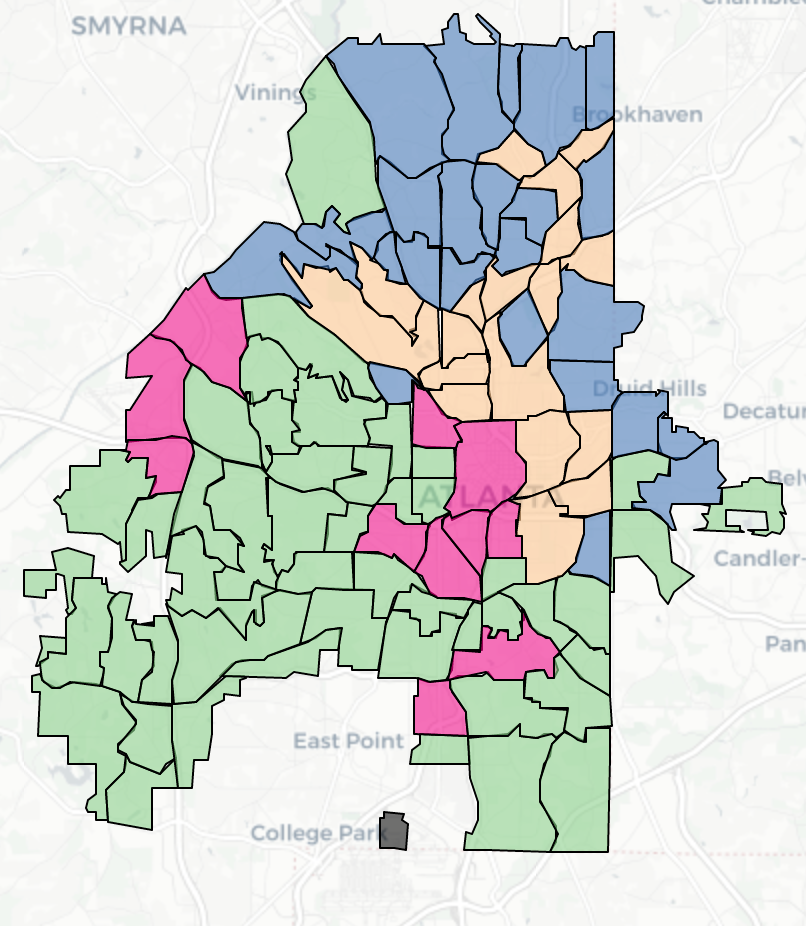
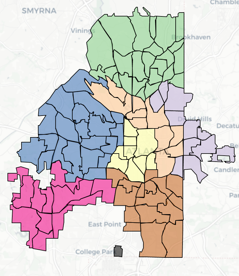
We refined the dataset by selecting variables with a standard deviation greater than 0.01 and applied K-means clustering to categorize neighborhoods based on crime patterns. The optimal number of clusters was determined to be K=4 using the elbow method. The neighborhoods within the same cluster were grouped into police patrol zones.
Optimization
We formulated a Mixed-Integer Linear Program (MILP) to minimize the distance between candidate police station locations and crime sites. Potential station sites were selected at the intersections of a mile-wide grid overlaying each patrol zone. Crimes were categorized into violent and non-violent incidents, weighted at 0.7 and 0.3, respectively, to prioritize proximity to violent crime locations.
\[ minimize \sum_{i \in I} x_i \left( \sum_{j \in J} 0.7 \times D_{H_{ij}} + \sum_{k \in K} 0.3 \times D_{L_{ik}} \right) \]
Subject to:
\[ \sum_{i \in I} x_i = n \]
The binary variable \( x_i \) indicates whether a candidate location \( i \) is selected for a police station. The parameter \( D_{H_{ij}} \) represents the distance from location \( i \) to crime site \( j \), while \( D_{L_{jk}} \) measures the distance from \( j \) to crime site \( k \). The parameter \( n \) represents the required number of police stations for each patrol zone.
4. Evaluation
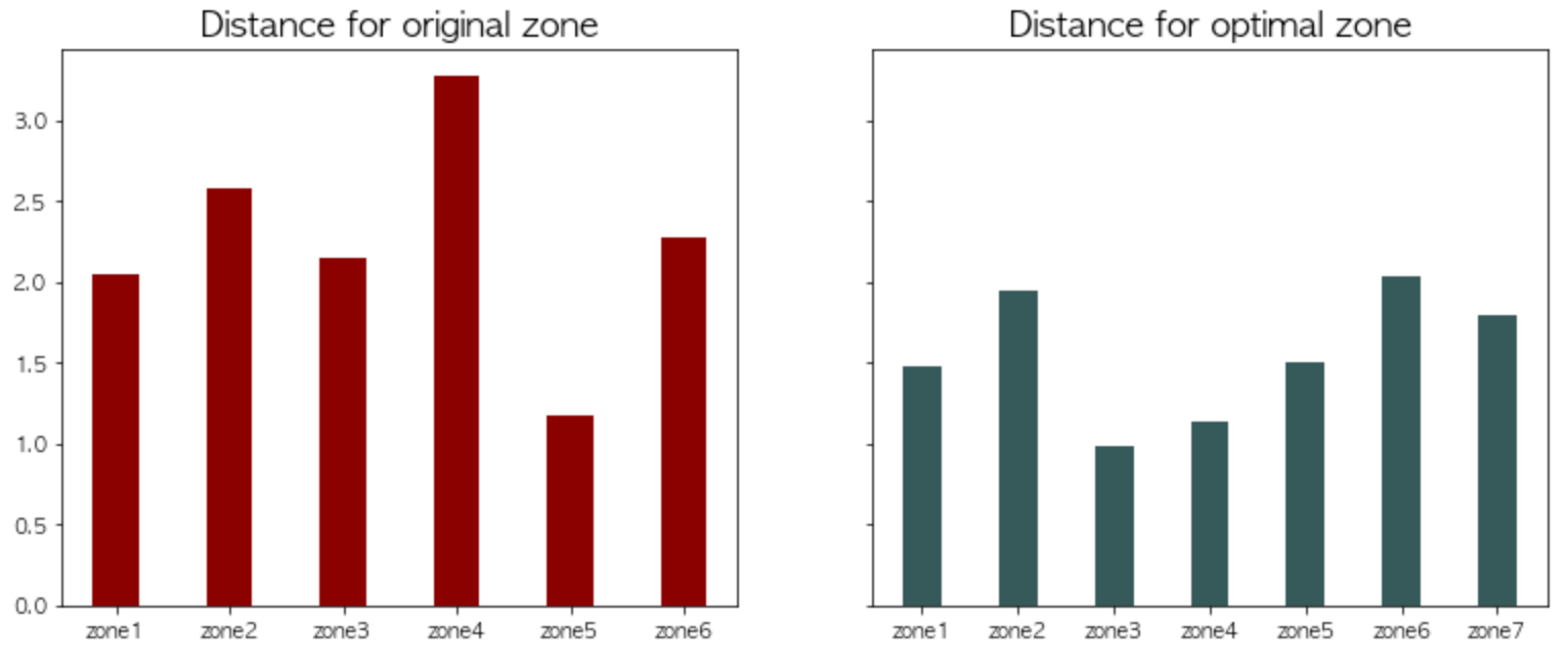
The optimization successfully reduced the average response distance by 40%, leading to a more efficient deployment of law enforcement resources. The model demonstrated that strategic station placement significantly enhances police presence in high-crime areas while minimizing overall travel time.